Identifying risky stocks

One of the ways to estimate how risky a stock is at some time is by looking at volatility. Stock volatility can be quantified as the standard deviation of the stock price relative to its average. Standard deviation is a statistical measure that tells you how much individual array elements deviate from the average. To estimate volatility, we’ll implement functions to compute average and standard deviation given an arbitrary input array. Furthermore, we’ll compute these metrics over a limited time window, and we’ll slide that window along the whole time series. This is the so-called moving average. For example, figure 5.3 shows the actual price, 30-day moving average, and volatility based on the 30-day moving standard deviation for Nvidia stock.

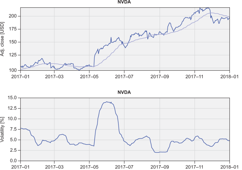
Figure 5.3 Top: Nvidia stock price (black) and a 30-day simple moving average (gray). Bottom: Volatility expressed as standard deviation relative to the 30-day simple moving average, in percent.

While Fortran comes with many built-in mathematical functions, it doesn’t include a function to compute the average of an array. That’s fairly straightforward to implement using the built-in functions sum and size, as shown in the following listing.

Listing 5.11 Computing the average value of an array

pure real function average(x)
  real, intent(in) :: x(:)
  average = sum(x) / size(x)      ❶
end function average

❶ The sum of all elements divided by the number of elements

We already saw earlier that we can use size in a do loop when we want to iterate over all elements of an array, or when we want to reference the last element of an array. sum does exactly what you think it does–you pass to it an array, and it returns the sum of all elements.

To calculate the standard deviation of an array x, follow these steps:

1. Calculate the average of the array –For this, use the function that we just wrote: average(x). The result is a scalar (nonarray).
2. Find the difference between each element of the array and its average –This is where the power of whole-array arithmetic comes in. We can use the subtraction operator - that we’re familiar with and apply it directly on the whole array, without the need for a loop: x - average(x). When using arithmetic (+, -, *, /, **), assignment (=), or comparison (>, >=, <=, <, ==, /=) operators, they’re applied element-wise. In this case, x is an array, and average(x) is a scalar; x - average(x) will subtract average(x) from each element of x. The result is an array.
3. Square the differences –This operates the same as in step 2, except this time we need to take the power of 2: (x - average(x)) ** 2. In this expression, ** is the power (exponentiation) operator.
4. Calculate the average of the squared differences –We can apply the same function again: average((x - average(x))**2).
5. Finally, take the square root of the result from step 4 –For this, we can use the built-in sqrt function, which is also an elemental function–it works on both scalars and arrays.

Here’s the complete code for the standard deviation function. Thanks to Fortran’s whole-array arithmetic, we can express all five steps as a one-liner, as shown in the following listing.

Listing 5.12 Computing the standard deviation of an array

pure real function std(x)
  real, intent(in) :: x(:)
  std = sqrt(average((x - average(x))**2))     ❶
end function std

❶ Root of mean squared differences

To use arithmetic operators on whole arrays, the arrays on either side of the operator must be of the same shape and size. You can also combine an array of any shape and size with a scalar. For example, if a is an array, 2 * a will be applied element-wise; that is, each element of a will be doubled.

Tip Use whole-array arithmetic over do loops whenever possible.

We’re not done here yet. Rather than just the average and standard deviation of the whole time series, we’re curious about the metrics that are relevant to a specific time, and we want to be able to see how they evolve. For this, we can use the average and standard deviation along a moving time window. A commonly used metric in finance is the so-called simple moving average, which takes an average of some number of previous points, moving in time. I’ll let you tackle this one in the “Exercise 3” sidebar, and will meet you on the other side.

Exercise 3: Calculating moving average and standard deviation

Our current implementations for average and standard deviation are great, but they don’t let us specify a narrow time period that would give us more useful information about stock volatility at a certain time.

Write a function, moving_average, that takes an input real array, x, and integer window, w, and returns an array that has the same size as x, but with each element being an average of w previous elements of x. For example, for w = 10, the moving average at element i would be the average of x(i-10:i). In finance, this is often referred to as the simple moving average.

Hint: You can use the built-in function max to limit the indices near the edges of x to prevent going out of bounds. For example, max(i, 1) results in i if greater than 1, and 1 otherwise. Note that you’ll need to use a combination of looping and whole-array arithmetic to implement the solution.

You can find the solution in the “Answer key” section near the end of the chapter.

The main program of this challenge is very similar to the previous one (stock_gain). However, besides printing the total time series average and volatility on the screen, now we also write the 30-day moving average and standard deviation into text files, as shown in the following listing.

Listing 5.13 Calculating stock volatility using moving average and standard deviation

program stock_volatility
 
  use mod_arrays, only: average, std, moving_average,&    ❶
                        moving_std, reverse               ❶
  use mod_io, only: read_stock, write_stock               ❶
  ...
  do n = 1, size(symbols)
    ...
    im = size(time)
    adjclose = reverse(adjclose)
    ...
    call write_stock(                        &            ❷
      trim(symbols(n)) // '_volatility.txt', &            ❷
      time(im:1:-1), adjclose,               &            ❷
      moving_average(adjclose, 30),          &            ❷
      moving_std(adjclose, 30))                           ❷
 
  end do
 
end program stock_volatility

❶ Accesses custom functions from modules

❷ Writes the 30-day moving average and standard deviation to files

Look inside src/mod_io.f 90 to see how the write_stock subroutine is implemented. The full program is located in src/stock_volatility.f 90.