Can we use historical stock market data to determine a good time to buy or sell shares of a stock? One of the commonly used indicators by traders is the moving average crossover. Consider that the simple moving average is a general indicator of whether the stock is going up or down. For example, a 30-day simple moving average would tell you about the overall stock price trend. You can think of it as a smoother and delayed stock price, without the high-frequency fluctuations. Combined with the actual stock price, we can use this information to decide whether we should buy or sell, or do nothing–see figure 5.4.
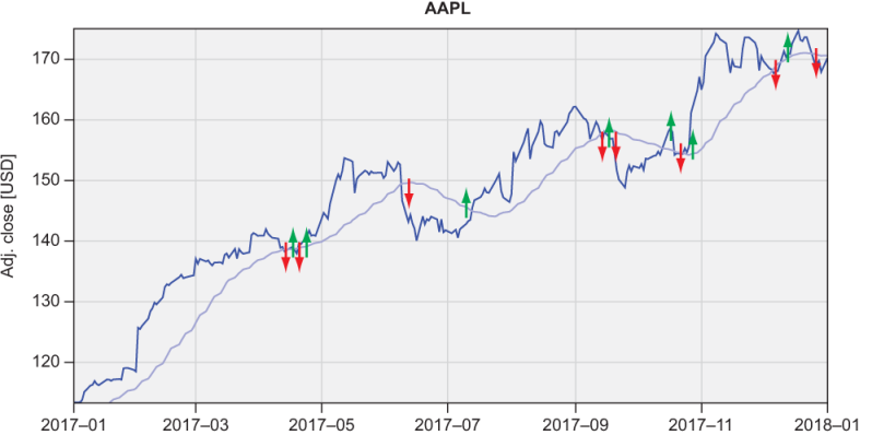
Figure 5.4 Moving average crossover indicators for Apple. Black is the adjusted daily closing price, gray is the 30-day simple moving average, and up and down arrows are the positive and negative crossover markers, respectively.
In this figure, I’ve marked with an up arrow every point in time when the actual price crossed the moving average line from low to high, and with a down arrow when crossing from high to low. The rule of thumb is this: sell when the actual price drops below the moving average line, buy when it rises above the moving average line.
Let’s employ Fortran arrays and arithmetic to compute the moving average crossover. The calculation has two steps:
- Compute the moving average over some time period. It can be any period of time, depending on the trends that you’re interested in (intra-day, short-term, long-term, etc.) and the frequency of the data that you have. We’re working with daily data, so we’ll work with a 30-day moving average. Hopefully, you worked through exercise 3 in the previous subsection and implemented the
moving_averagefunction. Otherwise, you can find it in src/mod_arrays.f 90. - Once we have the moving average, we can follow the actual stock price and find times when it crosses the moving average line. If the actual price crosses the moving average from below going up, it’s an indicator of a potentially good time to buy. Otherwise, if it crosses from above going down, it’s likely a good time to sell.
The main trick we’ll use for this challenge is to determine all array indices where the stock price is greater than its moving average, as well as those where the stock price is smaller than its moving average. We can then combine these two conditions and find all the indices where the stock price changes from smaller to greater, and vice versa. Figure 5.5 illustrates this algorithm.
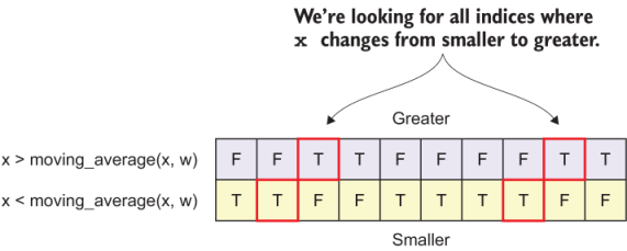
Figure 5.5 Finding indices where the stock price crosses its moving average
To implement this calculation, we’ll use almost all of the array features that we’ve learned about in this chapter so far: assumed-shape and dynamic array declaration, array constructor, and invoking a custom array function (moving_average). Furthermore, we’ll create logical (Boolean) arrays to handle the conditions I described in figure 5.5. Finally, we’ll employ a built-in function, pack, to select only those indices that satisfy our criteria.
We can write all this in about a dozen lines of code, as the following listing demonstrates.
Listing 5.14 Computing the moving-average crossover, low to high
pure function crosspos(x, w) result(res)
  real, intent(in) :: x(:)
  integer, intent(in) :: w
  integer, allocatable :: res(:)                  ❶
  real, allocatable :: xavg(:)                    ❷
  logical, allocatable :: greater(:), smaller(:)  ❸
  integer :: i
  res = [(i, i = 2, size(x))]                     ❹
  xavg = moving_average(x, w)                     ❺
  greater = x > xavg                              ❻
  smaller = x < xavg                              ❻
  res = pack(res, greater(2:) &                   ❼
                  .and. smaller(:size(x)-1))      ❼
end function crosspos
❶ We don’t know the size ahead of time, so we’ll declare this as a dynamic array.
❷ Array to store the moving average of x
❸ Logical (Boolean) arrays to mask x
❹ First guess result, all indices but the first
❻ Logical arrays to tell us where x is greater or smaller
❼ Uses built-in function pack to subset an array according to a condition
We first initialize our result array, res, as an integer sequence from 2 to size(x). This is our first guess from which we’ll subset only those elements that satisfy our criteria. The crux is in the last executable line, where we invoke the pack function. How does pack work? When you have an array x that you want to subset according to some condition mask, invoking pack(x, mask) will, as a result, return only those elements of x where mask is true. mask doesn’t have to be a logical array variable–it can be an expression as well, which is how we used it in our function in the listing. Recall the automatic reallocation on assignment from section 5.2.5? This is exactly where it comes in handy–we pass the original array, res, and a conditional mask to pack, and it returns a smaller, reallocated array, res, according to the mask.
This function only returns the crossover from low to high value, thus named crosspos. However, we also need the crossover from high to low so that we know when the stock price is going to drop below the moving average curve. How would we implement the negative variant of the crossover function, crossneg? We can reuse all the code from crosspos except for the last criterion–we need to look for elements that are going from higher to lower, instead of lower to higher:
pure function crossneg(x, w) result(res)
  ...
  res = pack(res, smaller(2:) .and. greater(:size(x)-1))     ❶
end function crossneg+
❶ Different criterion for the mask
The main program will use these functions to find the indices from the time series, and write the matching timestamps into files, as shown in the following listing.
Listing 5.15 Finding the moving average crossover times and writing them into files
program stock_crossover
  ...
  use mod_arrays, only: crossneg, crosspos, reverse      ❶
  ...
  integer, allocatable :: buy(:), sell(:)                ❷
  ...
  do n = 1, size(symbols)
    ...
    time = time(size(time):1:-1)                         ❸
    adjclose = reverse(adjclose)                         ❹

    buy = crosspos(adjclose, 30)                         ❺
    sell = crossneg(adjclose, 30)                        ❺

    open(newunit=fileunit, &                             ❻
         file=trim(symbols(n)) // '_crossover.txt')      ❻
    do i = 1, size(buy)
      write(fileunit, fmt=*) 'Buy ', time(buy(i))        ❼
    end do
    do i = 1, size(sell)
      write(fileunit, fmt=*) 'Sell ', time(sell(i))      ❽
    end do
    close(fileunit)                                      ❾

  end do

end program stock_crossover
❶ Accesses new functions from a module
❷ Integer indices for storing the crossovers
❸ Time is an array of strings, so we have to use the slice.
❹ Reverses using our custom function
❺ Finds the positive and negative crossover
❻ Opens the file to store the results
❼ Writes the positive crossover timestamps
❽ Writes the negative crossover timestamps
I included only the relevant new code in listing 5.15. The full program is located in src/stock_crossover.f 90. The program itself doesn’t do much new stuff. For each stock, it calls the moving average crossover functions, stores the results into arrays (buy and sell), and writes the timestamps with these indices into a text file. I plotted the results for Apple (AAPL) for 2017 in figure 5.4. You can use the Python scripts included in the repository to plot the results for other stocks and time periods.
Both the second and third challenge in this chapter produce results that I’ve plotted and showed in this section. The Python plotting scripts that I used are included in the stock-prices/plotting directory. Follow the directions in README.md to set up your own Python plotting environment. If you decide to further explore the stock prices data, you can use and modify these scripts for your own application.
And that’s it, we made it! Following only a few rules for array declaration, initialization, indexing, and slicing, we wrote a nifty little stock analysis app that tells us some useful things about the longer term trends and risk of individual stock prices. The skills that you learned in this chapter will form a foundation for what’s coming in chapter 7.