To go from uniform motion to a more realistic fluid flow, we need to add a few terms to the equations in our simulation code. Let’s briefly look at the shallow water equations that I first introduced in chapter 1 (figure 4.5). If you don’t care for the math, don’t worry about it; you can skip ahead to the next section, where we delve into the implementation.
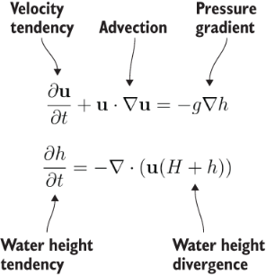
Figure 4.5 Shallow water equations revisited. The top equation is for water velocity, and the bottom for water height. We’ve already solved for the (linear) advection term.
We’re almost there! We already have the advection calculation, which allows the shape to move due to background flow. However, our water is currently moving like a solid object, and that’s what advection does–it simply moves things around in space. For the water to flow and slosh in response to gravity, much like real water would in a bathtub, we need to add the pressure gradient term. This term is proportional to gravitational acceleration multiplied by the slope of the water surface. The steeper the surface, the more it will accelerate in the horizontal direction. If the water rushes in from both sides, the water level will go up, and that’s what the water height divergence term does. The upside-down triangle symbol is called nabla and is the vector calculus symbol for the spatial gradient (difference in space). All the terms other than the tendency terms use this same operator! With some forethought, we designed our module so that we can reuse the finite difference function diff to add the remaining terms:
- The pressure gradient can now be expressed as
-g*diff(h)/dx. When the water surface is steep, this term makes the water rush forward, like in a breaking wave. We’ll add this term to our equation for velocity. - The water height divergence, which we can now write as
-diff(u*(hmean+h))/dx, acts to decrease the water height when the water mass is diverging (moving apart) or increase it when the water mass is converging (coming together). Think of a leaky bucket and the water level in it going down as the water comes out the bottom.
The structure of the new version of our app is illustrated in figure 4.6.
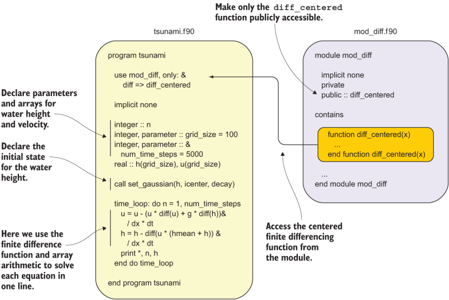
Figure 4.6 A diagram summarizing the structure of the one-dimensional tsunami simulator. The main program is shown on the left, and the supporting module is shown on the right. Only the key parts of the code are shown.