Recall that in the previous version of the tsunami simulator, we did quite a lot of prep work before allocating the data arrays. Now that we know how to write a custom constructor, let’s apply this technique to initializing the Field type. For the time being, let’s focus on just finding the start and end indices, allocating the data array, and initializing its values.
Continuing from where we left off in section 8.2.1, we’ll now add two more integer components to keep track of the lower and upper bounds of the array, and a real, two-dimensional array to hold the actual values of the field:
type :: Field
  character(len=:), allocatable :: name
  integer(int32) :: dims(2), lb(2), ub(2)     ❶
  real(real32), allocatable :: data(:,:)      ❷
end type Field
❶ Tracks the global array size and lower and upper bounds of this tile
❷ Dynamic 2-D array to hold the field values
Relative to the earlier Field definition, we now have three additional components: integer length-2 arrays lb and ub to represent lower and upper array bounds, respectively, and the data array itself, the allocatable two-dimensional array of real numbers. The goal for our custom constructor is to compute the lower and upper bounds given input dimensions dims, use these bounds to allocate the array data(:,:) with correct extents (start and end indices), and initialize it to zero. Figure 8.5 illustrates the relationship between the global dimensions dims = [im, jm] and lower and upper bounds (lb and ub, respectively) of the array after the parallel decomposition of the domain.
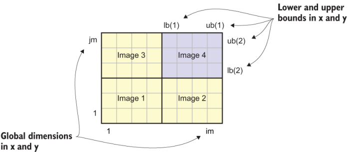
Figure 8.5 Global dimensions and local bounds in a parallel decomposition of a two-dimensional field
The large rectangle in figure 8.5 represents the whole domain that the tsunami simulator is solving for. This domain extends from 1 to im in the x direction and from 1 to jm in the y direction. When decomposed between four parallel images, each tile extends from lb(1) to ub(1) in the x direction, and from lb(2) to ub(2) in the y direction. The following listing shows the first version of our new constructor.
Listing 8.6 Adding lower and upper bound indices and field values to the components
type(Field) function field_constructor(name, dims) result(res)
  character(len=*), intent(in) :: name
  integer(int32), intent(in) :: dims(2)
  integer(int32) :: indices(4)                         ❶
  res % name = name                                    ❷
  res % dims = dims                                    ❷
  indices = tile_indices(dims)                         ❸
  res % lb = indices([1, 3])                           ❹
  res % ub = indices([2, 4])                           ❹
  allocate(res % data(res % lb(1)-1:res % ub(1)+1,&    ❺
                      res % lb(2)-1:res % ub(2)+1))    ❺
  res % data = 0                                       ❻
end function field_constructor
❶ Temporary integer array to store start and end indices
❷ Assigns input name and dimensions to type components
❸ Calculates local tile indices using an external function
❹ Assigns lower and upper bounds
This constructor function does a few things. First, we pass the field name and domain dimensions (dims) as arguments, and these are assigned to its respective components, res % name and res % dims. If we left it at this, the constructor would be semantically equivalent to the default constructor from section 8.2.1. However, now that we intend to allocate the data array, we need to do a few more operations.
The second step is to determine the lower and upper bounds for the local image. Recall from the previous chapter that at the beginning of the tsunami program, we break the domain down into pieces and assign each piece to all available images. The local array extents will thus be different for each parallel image, like tiles on a chess board. These extents are calculated in the tile_indices function. We’ve already worked with the one-dimensional variant of this function, and here we apply it for a two-dimensional array. Its implementation is a bit more complex, and you can find it in appendix C.
Finally, once we have the start and end indices computed and stored in res % lb (lower bounds) and res % ub (upper bounds), respectively, we can use them to allocate the data array, res % data. In the allocate statement, we give one extra point on each end to account for the halo exchange. Once allocated, we initialize the array to zero to avoid potential undefined behavior due to uninitialized array values.
Notice that we’ve carefully designed our custom constructor such that we can still create a Field instance in the same way as we did at the end of section 8.2.2. Here’s an example initialization of fields for water height and velocity with global dimensions of [im, jm]:
h = Field('Water height', [im, jm])
u = Field('Water velocity in x', [im, jm])
v = Field('Water velocity in y', [im, jm])
If the benefits of derived types for our tsunami simulator haven’t been obvious before, they should be now. Whereas before we had to calculate lower and upper bounds and explicitly use them to allocate arrays in memory, this is now all done under the hood for each Field instance that we create. This becomes especially powerful once we do significantly more work in the constructor. If you take a look at the code for the Field constructor in src/ch08/mod_field.f 90, you’ll see that we actually need to do a few more things related to the parallel decomposition of the field, which I haven’t covered in this section for brevity. Feel free to explore the code, but know that we’ll revisit this in chapter 10 when we finish the implementation of the Field class.