Before we start refactoring the solver for parallel execution, let’s refresh our memory about where we left off.
Relative to the top-level directory of the project, the main program is located in src/ch04/tsunami.f 90. The core of our solver is the do loop to integrate the solution in time:
time_loop: do n = 1, num_time_steps               ❶

  u = u - (u * diff(u) + g * diff(h)) / dx * dt   ❷

  h = h - diff(u * (hmean + h)) / dx * dt         ❸

  print *, n, h                                   ❹

end do time_loop❹ Writes the water height array to screen
As we saw in chapter 3, assignments for velocity u and water height h are whole-array operations, and we don’t need to loop over the elements. Hopefully, we should be able to do the same in parallel mode, except that each image will work on its own section of the array. Now, recall what we did in section 7.3 where we parallelized the weather buoy program. We divided the input array into a number of equal parts, a number that matched the total number of images. Then we did the core calculation in the same way as we did in the serial version of the program. Let’s apply the same strategy here, keeping in mind that we need to send, receive, and synchronize data at every step of the time_loop. This is because at each time step, the spatial difference function diff will need nonlocal data that belong to neighbor images, as shown in figure 7.9.
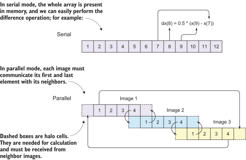
Figure 7.9 Communicating data between neighbor images. The numbers in each box are array indices. Each image computes the solution for the elements in solid boxes; however, values from dashed boxes are needed for the computation and must be received from neighbor processors. The far-end communication between images 1 and 3 is to satisfy the periodic boundary condition.
Recall from src/ch04/mod_diff.f 90 how our difference function works:
do concurrent(i = 2:im-1)              ❶
  dx(i) = 0.5 * (x(i+1) - x(i-1))      ❷
end do
❶ Loops over all elements except first and last
❷ Takes centered difference in space
Each element of the result of the diff function depends on the elements immediately next to it. This is a classic example of a nonembarrassingly parallel (or communication-intensive) function, in which we have to send and receive data between neighbor images before doing the calculation. To better understand why, see figure 7.9.
In serial mode (figure 7.9, top), array indices go from 1 to the total size of the array (12, in this case), and there’s no distinction between global and local indices. In parallel mode (figure 7.9, bottom), each image holds a subsection of the array, with local indices going from 1 to the total size of the subsection of the array (4, in this case). Each local index maps to a unique global index: local indices 1-4 on images 1, 2, and 3 map to global indices 1-4, 5-8, and 9-12, respectively.
When invoking the diff(x) function, the calculation of each array element x(i) depends on the two elements immediately next to it: x(i-1) and x(i+1). What happens on image 2 when we try to calculate the difference for element 5? We need elements 4 and 6, but the problem is that element 4 is computed by image 1, so image 2 doesn’t have it in its local memory! This is a new challenge that we didn’t encounter before, and it requires performing the communication pattern before each invocation of the diff function.
This is where the concept of halo cells becomes useful. Halo cells refer to array elements that belong to neighbor images, but are needed locally to perform the calculation. In the example of the diff function, if index i points to the first array element on the local image, x(i-1), which belongs to a neighbor image, must be received and stored into an array element on the local image.
Another important concept to understand is that of global and local indices. Global indices are the array indices that cover the whole array, like in the serial program. In figure 7.9, global indices go from 1 to 12. Local indices are the indices of the array subsets that each image sees in its local memory. In this case, the local indices go from 1 to 4 on each of the three images. However, to accommodate halo cells, we need to add one element on both ends, so the local indices in memory will go from 0 to 5, but only elements 1 through 4 will be computed locally.
To make the tsunami simulator work in parallel, each image must carry out the following steps:
- Determine neighbor images.
- Determine start and end indices on each image, and allocate the coarrays accordingly.
- Update the halo cells and compute the solution.
Let’s go over these steps one at a time. You can follow the next few subsections and build the parallel code together with me if you want.