Finally, we’ve gotten to the exciting part: taking the pieces that we’ve learned and putting them together into a complete and working program. We’ll first look at the solution of our program, visualized with a Python script, and then go through the complete code.
The result
The numerical solution of our simple app is shown in figure 2.7. From top to bottom, each panel shows the state of water height at increments of 25 time steps. The top panel corresponds to the initial condition, as in figure 2.6. The position of the water height peak in each panel is consistent with the configuration of the physical parameters of the simulation: background flow speed (c = 1), grid spacing (dx = 1), and time step (dt = 1). In the bottom panel, we can see the water height peak moving out on the right and reentering on the left. This confirms that our periodic boundary condition works as intended.
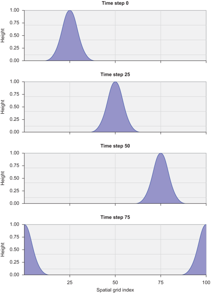
Figure 2.7 Predicting the linear advection of an object, with periodic boundary conditions. The water height perturbation is advected from left to right with a constant speed of 1 m/s. When the water reaches the boundary on the right, it reenters the domain from the left.
Although Fortran is great for high-performance numerical work, it’s less elegant for graphics and visualization of data. For brevity and simplicity, I use Python scripts for visualization of the tsunami results. You can find the visualization code in the tsunami repository on GitHub (https://github.com/modern-fortran/tsunami), alongside the Fortran source code in each chapter directory.
Complete code
The complete code for the first version of our tsunami simulator is given in the following listing.
Listing 2.14 Complete code of the minimal working tsunami simulator
program tsunami                                           ❶

  implicit none                                           ❷

  integer :: i, n                                         ❸
                                                          ❸
  integer, parameter :: grid_size = 100                   ❸
  integer, parameter :: num_time_steps = 100              ❸
                                                          ❸
  real, parameter :: dt = 1 ! time step [s]               ❸
  real, parameter :: dx = 1 ! grid spacing [m]            ❸
  real, parameter :: c = 1 ! background flow speed [m/s]  ❸
                                                          ❸
  real :: h(grid_size), dh(grid_size)                     ❸
                                                          ❸
  integer, parameter :: icenter = 25                      ❸
  real, parameter :: decay = 0.02                         ❸

  if (grid_size <= 0) stop 'grid_size must be > 0'        ❹
  if (dt <= 0) stop 'time step dt must be > 0'            ❹
  if (dx <= 0) stop 'grid spacing dx must be > 0'         ❹
  if (c <= 0) stop 'background flow speed c must be > 0'  ❹

  do concurrent(i = 1:grid_size)
    h(i) = exp(-decay * (i - icenter)**2)                 ❺
  end do

  print *, 0, h                                           ❻

  time_loop: do n = 1, num_time_steps                     ❼

    dh(1) = h(1) - h(grid_size)                           ❽

    do concurrent (i = 2:grid_size)
      dh(i) = h(i) - h(i-1)                               ❾
    end do

    do concurrent (i = 1:grid_size)
      h(i) = h(i) - c * dh(i) / dx * dt                   ❿
    end do

    print *, n, h                                         ⓫

  end do time_loop

end program tsunami❷ Enforces explicit declaration of variables
❹ Checks input parameter values and aborts if invalid
❺ Loops over array elements and initializes values
❻ Writes the initial water height values to the terminal
❽ Applies the periodic boundary condition at the left edge of the domain
❾ Calculates the finite difference of water height in space
❿ Integrates the solution forward; this is the core of our solver
⓫ Prints current values to the terminal
With only 30 lines of code, this is a useful little solver! If you compile and run this program, you’ll get a long series of numbers as text output on the screen, as shown in the following listing.
Listing 2.15 Text output of the current version of the tsunami simulator
0   9.92950936E-06   2.54193492E-05   6.25215471E-05  ...     ❶
1   0.00000000       9.92950845E-06   2.54193510E-05  ...     ❷
2   0.00000000       0.00000000       9.92950845E-06  ...     ❸
...❷ Output after first time step
❸ Output after second time step
Although it may look like nonsense, these are our predicted water height values (in meters). However, the output is long and will flood your terminal window. You’ll be able to explore the output more easily if you redirect it to a file, as the following listing demonstrates.
Listing 2.16 Building, running, and visualizing the output from the tsunami simulator
cd src/ch02                                             ❶
gfortran tsunami.f90 -o tsunami                         ❷
./tsunami > tsunami_output.txt                          ❸
python3 plot_height_multipanel.py tsunami_output.txt    ❹
❶ Enters the source code directory
❸ Runs the program and redirects the output into a text file
❹ Visualizes the output and writes it to an image file
Alternatively, the source code repository on GitHub also comes with a Makefile to streamline the build process, and you can type make ch02 from the top-level directory. This also assumes that you’ve set up the Python virtual environment following the instructions in the README.md file in the repository.
Go ahead and play with it. Some ideas that come to mind:
- Tweak the initial conditions, perhaps by changing the shape and position of the initial perturbation. For example, you can change the values of the
decayandicenterparameters, or use a different function when initializing theharray. Try a sine wave (intrinsic functionsin). - Change the grid size and number of time steps parameters.
Remember that Fortran is a compiled language. Every time you change the code, you’ll need to recompile it before running it.