In the previous chapter, we made the first working version of what will become a realistic water wave simulator. Contained in a single program, it included data declaration and initialization, arithmetic expressions and assignment to calculate the solution, a do loop to advance the solution forward in time, and a print statement to output the results to screen. With 26 lines of code, this is a simple program that does simple things: it initializes the water height, simulates its movement forward due to background flow, and writes its state to the screen at each time step (figure 3.1).
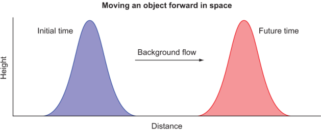
Figure 3.1 Advecting a Gaussian shape in space from left to right. We worked on this problem in the previous chapter.
In this chapter, we’ll refactor the simulator to use a set of common building blocks, such as the finite difference calculation that I introduced in chapter 2. This will allow us to more easily expand the simulator in the following chapters as we move toward a more realistic water wave motion. Recall the core of our solver from the previous chapter, shown in the following listing.
Listing 3.1 Time integration loop from the minimal working tsunami simulator
time_loop: do n = 1, num_time_steps     ❶

  dh(1) = h(1) - h(grid_size)           ❷

  do concurrent (i = 2:grid_size)       ❸
    dh(i) = h(i) - h(i-1)               ❸
  end do                                ❸

  do concurrent (i = 1:grid_size)       ❹
    h(i) = h(i) - c * dh(i) / dx * dt   ❹
  end do                                ❹

end do time_loop
❶ Iterates for num_time_steps time steps
❷ Calculates the difference on the left boundary
❸ Calculates the difference in the rest of the domain
❹ Computes and stores the value of h at the next time step
The body of the main loop (time_loop) consists of two steps: calculating the difference of water height h in space, and using that difference to predict and store its new value at the next time step. This solves for only one equation for water height, which features one physics term, namely the linear advection.
To add more terms and another equation, we’ll define a new array, u, for the water velocity and add any calculations inside time_loop to make the solver complete. Without assuming anything about what the equations or the code should look like, figure 3.2 illustrates the tentative update of our app.
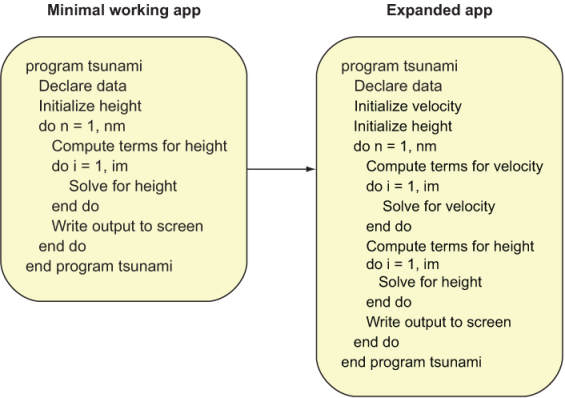
Figure 3.2 Expanding the minimal working app to a more realistic simulator
The key operations we were doing to simulate the evolution of water height–initialization, calculating the change in time, and solving the equation–we’d now be doing for both water height and velocity. It looks like our program would at least double in size if we added code to solve for another variable. Furthermore, if we added more terms to each of the equations, our program would grow further. It’s clear that our program will inevitably become difficult to work with if we keep piling more and more code on top of it.
In the previous chapter, you learned that most of the computational work in fluid dynamics boils down to approximating partial derivatives with a discrete form that can be expressed as code. Finite differences, which we used to calculate the gradient of the water surface to predict its movement due to advection, are what we’ll use for all the other terms in the tsunami simulator. Since we’ll spend most of the time (human and computer time!) on these terms, we should find a way to abstract this low-level calculation and make it reusable from the main solver loop. This is where Fortran procedures and modules come in (figure 3.3).
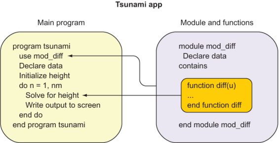
Figure 3.3 Using a module and a function to reuse and simplify code. Module mod_diff, which defines the difference function diff, is accessed from the main program with the use statement (top arrow). Through use association, the function diff can be used within the scope of the main program (bottom arrow).
In this new framework, we define the reusable data and functions inside the module. The module is then accessed from the main program with the use statement. We’ll first refactor our minimal working app to compute the finite difference in a function, while exactly reproducing the existing results. Then, in the next chapter, we’ll define our new custom module to host our functions, and we’ll expand our app to produce more realistic simulations.