Revisiting the cold front problem

In the previous chapter (section 2.2.2), I introduced the example of a cold front to illustrate the concepts of temperature gradient (change in space) and tendency (change in time). There, I asked you to calculate the change of temperature in Miami, considering the temperatures in Atlanta and Miami, the distance between them, and the speed of the front (figure 3.4).

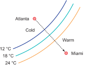
Figure 3.4 An illustration of a cold front moving from Atlanta toward Miami. Curved lines are contours of constant temperature. The dashed arrow shows the direction of front propagation. We used this example in the previous chapter to illustrate the concept of spatial gradients and advection.

What would the program that solves this problem look like? For simplicity, let’s assume the same initial parameters as in the example:

• The temperature is 12 °C in Atlanta, and 24 °C in Miami.
• The distance between Atlanta and Miami is 960 kilometers.
• The front is moving toward Miami at a constant speed of 20 km/h.

The compiled program should yield

Temperature after    24.0000000     hours is    18.0000000     degrees.

If you worked through the exercise of building the minimal working app in the previous chapter, then you have all the ingredients to solve this problem: defining the program unit, declaring and initializing data, basic arithmetic expression and assignment, and printing to screen. The following listing provides the complete code.

Listing 3.2 Solving for temperature due to passage of a cold front

program cold_front
 
  implicit none                                ❶
 
  real :: temp1 = 12, temp2 = 24               ❷
  real :: dx = 960, c = 20, dt = 24            ❷
  real :: res ! result in deg. C               ❸
 
  res = temp2 - c * (temp2 - temp1) / dx * dt  ❹
 
  print *, 'Temperature after ', dt, &         ❺
           'hours is ', res, 'degrees'         ❺
 
end program cold_front

❶ All declarations will be explicit.

❷ Declares and initializes the variables

❸ The variable to store the result in

❹ Computes the solution

❺ Writes the solution to screen

We first declared and initialized all the input parameters:

1. Origin and destination temperatures, temp1 and temp2, respectively
2. Distance in kilometers, dx
3. Front speed in kilometers per hour, c
4. Time interval in hours, dt
5. The variable res to store the result in

The calculation itself fits into a single expression and assignment.

This program works well if you need to do the calculation once or twice. However, what if the exercise required you to calculate the temperature for multiple different values of input parameters, be it temp1, temp2, dx, c, or dt? You can see where I’m going with this. Specifically, I could ask you to calculate the solution in the case of temp1 being 0 °C, another solution for a front speed of 28 km/h, or the solution after 36 hours. How would you solve this problem? You could compute the first solution, then reinitialize variables and compute another solution, and so on. However, this would soon become quite tedious and result in repetition of code. More problematically, how would you implement a solution that had to work with a continuous stream of input parameters in real time, such as those measured at real-world weather stations?

Experiment a bit

Try plugging in different values for input parameters and rerunning the program. (You’ll have to recompile it as well.) Do the results look reasonable? Also, can you find a value of any input parameter that breaks the program? Try it!