At this stage, we’ll simulate only the movement of an object (or fluid) due to background flow. This will provide the foundation for other physical processes that we’ll add to the solver in later chapters. Simulating only one process for now will guide the design of our program structure and its elements: declaration and initialization of data, iterating the simulation forward in time, and writing the results to the terminal. I sketched the result that we expect in figure 2.2.
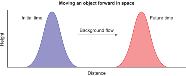
Figure 2.2 Advecting an object in space from left to right. The initial state is on the left. The object is advected from left to right by a background flow and after some time arrives at its final position on the right.
Note that the advected object can be any quantity, such as water height, temperature, or concentration of a pollutant. For now, we’ll just refer to it as the object for simplicity. The shape of the object is also arbitrary–it can be any continuous or discontinuous function. I chose a smooth bulge for convenience. At the initial time, the object is located near the left edge of the domain. Our goal is to simulate the movement of the object due to background flow and record the state of the object at some future time. Internally, our app will need to perform the following steps:
- Initialize –Define the data structure that will keep the state of the object in computer memory, and initialize its value.
- Simulate –This step will calculate how the position of the object will change over time. At this stage, we expect it only to move from left to right, without change in shape. The simulation is done over many discrete time steps and makes up for most of the compute time spent by the program.
- Output –At each time step, we’ll record the state of the object so that we can visualize it with an external program.
As you can guess, the core of our program will revolve around the simulation step. How do we go about simulating the movement of the object? Before writing any code, we need to understand how advection works.